How create bar chart race with python
Recently, I come across a medium post on announcement off Official Release of bar_chart_race by Ted Petrou. In his article, he provides an excellent tutorial on how to create Bar Chart Race using bar_chart_race package. Check out the official document here .
In our example we use a World Population from 1955 to 2020 dataset from kaggle or you can directly download dataset here .
Installation of Bar Chart Race package
pip3 install bar_chart_race pandas
or using anaconda:
conda install -c conda-forge bar_chart_race
conda install -c conda-forge pandas
Installing ffmpeg
In order to save animations as mp4/m4v/mov/etc... files, you must install ffmpeg , which allows for conversion to many different formats of video and audio. For macOS users, installation may be easier using Homebrew .
After installation, ensure that ffmpeg has been added to your path by going to your command line and entering ffmpeg -version.
Install ImageMagick for animated gifs
If you desire to create animated gifs, you'll need to install ImageMagick . Verify that it has been added to your path with magick -version.
Install fonts
Maybe you have to install fonts for debian distros:
~] apt-get install fonts-freefont-otf fonts-freefont-ttf
Import Required Libraries and Load dataset
import pandas as pd
import bar_chart_race as bcr

population = pd.read_csv('./datasets_countries_population_from_1995_to_2020.csv')
Edit dataset
In bar chart race, your data must be in a specific format:
-
each entry represents a single time
-
each feature have some single particular value
-
time should be set as .index
Let’s have a look at how our data is looking.
population.head()
#Output:
   Year Country  Population  Yearly % Change  Yearly Change  Migrants (net)  Median Age  Fertility Rate Density (P/Km²)  Urban Pop %  Urban Population  Country's Share of World Pop %  World Population  Country Global Rank
0  2020   China  1439323776             0.39        5540090       -348399.0        38.4            1.69             153         60.8       875075919.0                           18.47        7794798739                    1
1  2019   China  1433783686             0.43        6135900       -348399.0        37.0            1.65             153         59.7       856409297.0                           18.59        7713468100                    1
2  2018   China  1427647786             0.47        6625995       -348399.0        37.0            1.65             152         58.6       837022095.0                           18.71        7631091040                    1
3  2017   China  1421021791             0.49        6972440       -348399.0        37.0            1.65             151         57.5       816957613.0                           18.83        7547858925                    1
4  2016   China  1414049351             0.51        7201481       -348399.0        37.0            1.65             151         56.3       796289491.0                           18.94        7464022049                    1
So it’s clear that our data is not in the appropriate format to feed in bar_chart_race. First, make relevant changes in data.
Step 1: Remove all columns except Year, Country, and Population.
population = population.drop(['Yearly % Change', 'Yearly Change', 'Migrants (net)', 'Median Age', 'Fertility Rate', 'Density (P/Km²)', 'Urban Pop %', 'Urban Population', 'Country\'s Share of World Pop %', 'World Population', 'Country Global Rank'], axis=1)

population.head()
   Year Country  Population
0  2020   China  1439323776
1  2019   China  1433783686
2  2018   China  1427647786
3  2017   China  1421021791
4  2016   China  1414049351
Step 2: Create pivot_table from the pop data frame where Year is an index; each country as column and Population as value.
population = population.pivot_table('Population', ['Year'], 'Country')

population
>>> population
Country  Afghanistan    Albania     Algeria  American Samoa  Andorra      Angola  Anguilla  Antigua and Barbuda  ...   Vanuatu   Venezuela     Vietnam  Wallis & Futuna  Western Sahara       Yemen      Zambia    Zimbabwe
Year                                                                                                             ...
1955       8270991.0  1419994.0   9774283.0         19754.0   9232.0   5043247.0    5783.0              49648.0  ...   54921.0   6744695.0  28147443.0           7669.0         21147.0   4965574.0   2644976.0   3213286.0
1960       8996973.0  1636090.0  11057863.0         20123.0  13411.0   5454933.0    6032.0              54131.0  ...   63689.0   8141841.0  32670039.0           8157.0         32761.0   5315355.0   3070776.0   3776681.0
1965       9956320.0  1896171.0  12550885.0         23672.0  18549.0   5770570.0    6361.0              58698.0  ...   74270.0   9692278.0  37858951.0           8724.0         50970.0   5727751.0   3570464.0   4471177.0
1970      11173642.0  2150707.0  14464985.0         27363.0  24276.0   5890365.0    6771.0              64177.0  ...   85377.0  11396393.0  43404793.0           8853.0         76874.0   6193384.0   4179067.0   5289303.0
1975      12689160.0  2411732.0  16607707.0         30052.0  30705.0   7024000.0    7159.0              62675.0  ...   99859.0  13189509.0  48718189.0           9320.0         74954.0   6784695.0   4943283.0   6293875.0
1980      13356511.0  2682690.0  19221665.0         32646.0  36067.0   8341289.0    7285.0              61865.0  ...  115597.0  15182611.0  54281846.0          11231.0        150877.0   7941898.0   5851825.0   7408624.0
1985      11938208.0  2969672.0  22431502.0         39519.0  44600.0   9961997.0    7293.0              61786.0  ...  129984.0  17319520.0  60896721.0          13622.0        182421.0   9572175.0   6923149.0   8877489.0
1990      12412308.0  3286073.0  25758869.0         47347.0  54509.0  11848386.0    8899.0              62528.0  ...  146573.0  19632665.0  67988862.0          13800.0        217258.0  11709993.0   8036845.0  10432421.0
1995      18110657.0  3112936.0  28757785.0         53161.0  63850.0  13945206.0    9866.0              68670.0  ...  168158.0  21931084.0  74910461.0          14149.0        255634.0  14913315.0   9096607.0  11410714.0
2000      20779953.0  3129243.0  31042235.0         57821.0  65390.0  16395473.0   11252.0              76016.0  ...  184972.0  24192446.0  79910412.0          14694.0        314118.0  17409072.0  10415944.0  11881477.0
2005      25654277.0  3086810.0  33149724.0         59562.0  78867.0  19433602.0   12453.0              81465.0  ...  209282.0  26432447.0  83832661.0          14939.0        437515.0  20107409.0  11856247.0  12076699.0
2010      29185507.0  2948023.0  35977455.0         56079.0  84449.0  23356246.0   13438.0              88028.0  ...  236211.0  28439940.0  87967651.0          12689.0        480274.0  23154855.0  13605984.0  12697723.0
2015      34413603.0  2890513.0  39728025.0         55812.0  78011.0  27884381.0   14279.0              93566.0  ...  271130.0  30081829.0  92677076.0          12266.0        526216.0  26497889.0  15879361.0  13814629.0
2016      35383032.0  2886438.0  40551392.0         55741.0  77297.0  28842489.0   14429.0              94527.0  ...  278330.0  29851255.0  93640422.0          12107.0        538749.0  27168208.0  16363458.0  14030331.0
2017      36296113.0  2884169.0  41389189.0         55620.0  77001.0  29816766.0   14584.0              95426.0  ...  285510.0  29402484.0  94600648.0          11900.0        552615.0  27834819.0  16853599.0  14236595.0
2018      37171921.0  2882740.0  42228408.0         55465.0  77006.0  30809787.0   14731.0              96286.0  ...  292680.0  28887118.0  95545962.0          11661.0        567402.0  28498683.0  17351708.0  14438802.0
2019      38041754.0  2880917.0  43053054.0         55312.0  77142.0  31825295.0   14869.0              97118.0  ...  299882.0  28515829.0  96462106.0          11432.0        582463.0  29161922.0  17861030.0  14645468.0
2020      38928346.0  2877797.0  43851044.0             NaN      NaN  32866272.0       NaN              97929.0  ...  307145.0  28435940.0  97338579.0              NaN        597339.0  29825964.0  18383955.0  14862924.0
Step3: Sometimes your data is not in order, so make sure you order the time column. In our case, its Year.
population.sort_values(list(population.columns),inplace=True)
population = population.sort_index()
population
Country  Afghanistan    Albania     Algeria  American Samoa  Andorra      Angola  Anguilla  Antigua and Barbuda  ...   Vanuatu   Venezuela     Vietnam  Wallis & Futuna  Western Sahara       Yemen      Zambia    Zimbabwe
Year                                                                                                             ...
1955       8270991.0  1419994.0   9774283.0         19754.0   9232.0   5043247.0    5783.0              49648.0  ...   54921.0   6744695.0  28147443.0           7669.0         21147.0   4965574.0   2644976.0   3213286.0
1960       8996973.0  1636090.0  11057863.0         20123.0  13411.0   5454933.0    6032.0              54131.0  ...   63689.0   8141841.0  32670039.0           8157.0         32761.0   5315355.0   3070776.0   3776681.0
1965       9956320.0  1896171.0  12550885.0         23672.0  18549.0   5770570.0    6361.0              58698.0  ...   74270.0   9692278.0  37858951.0           8724.0         50970.0   5727751.0   3570464.0   4471177.0
1970      11173642.0  2150707.0  14464985.0         27363.0  24276.0   5890365.0    6771.0              64177.0  ...   85377.0  11396393.0  43404793.0           8853.0         76874.0   6193384.0   4179067.0   5289303.0
1975      12689160.0  2411732.0  16607707.0         30052.0  30705.0   7024000.0    7159.0              62675.0  ...   99859.0  13189509.0  48718189.0           9320.0         74954.0   6784695.0   4943283.0   6293875.0
1980      13356511.0  2682690.0  19221665.0         32646.0  36067.0   8341289.0    7285.0              61865.0  ...  115597.0  15182611.0  54281846.0          11231.0        150877.0   7941898.0   5851825.0   7408624.0
1985      11938208.0  2969672.0  22431502.0         39519.0  44600.0   9961997.0    7293.0              61786.0  ...  129984.0  17319520.0  60896721.0          13622.0        182421.0   9572175.0   6923149.0   8877489.0
1990      12412308.0  3286073.0  25758869.0         47347.0  54509.0  11848386.0    8899.0              62528.0  ...  146573.0  19632665.0  67988862.0          13800.0        217258.0  11709993.0   8036845.0  10432421.0
1995      18110657.0  3112936.0  28757785.0         53161.0  63850.0  13945206.0    9866.0              68670.0  ...  168158.0  21931084.0  74910461.0          14149.0        255634.0  14913315.0   9096607.0  11410714.0
2000      20779953.0  3129243.0  31042235.0         57821.0  65390.0  16395473.0   11252.0              76016.0  ...  184972.0  24192446.0  79910412.0          14694.0        314118.0  17409072.0  10415944.0  11881477.0
2005      25654277.0  3086810.0  33149724.0         59562.0  78867.0  19433602.0   12453.0              81465.0  ...  209282.0  26432447.0  83832661.0          14939.0        437515.0  20107409.0  11856247.0  12076699.0
2010      29185507.0  2948023.0  35977455.0         56079.0  84449.0  23356246.0   13438.0              88028.0  ...  236211.0  28439940.0  87967651.0          12689.0        480274.0  23154855.0  13605984.0  12697723.0
2015      34413603.0  2890513.0  39728025.0         55812.0  78011.0  27884381.0   14279.0              93566.0  ...  271130.0  30081829.0  92677076.0          12266.0        526216.0  26497889.0  15879361.0  13814629.0
2016      35383032.0  2886438.0  40551392.0         55741.0  77297.0  28842489.0   14429.0              94527.0  ...  278330.0  29851255.0  93640422.0          12107.0        538749.0  27168208.0  16363458.0  14030331.0
2017      36296113.0  2884169.0  41389189.0         55620.0  77001.0  29816766.0   14584.0              95426.0  ...  285510.0  29402484.0  94600648.0          11900.0        552615.0  27834819.0  16853599.0  14236595.0
2018      37171921.0  2882740.0  42228408.0         55465.0  77006.0  30809787.0   14731.0              96286.0  ...  292680.0  28887118.0  95545962.0          11661.0        567402.0  28498683.0  17351708.0  14438802.0
2019      38041754.0  2880917.0  43053054.0         55312.0  77142.0  31825295.0   14869.0              97118.0  ...  299882.0  28515829.0  96462106.0          11432.0        582463.0  29161922.0  17861030.0  14645468.0
2020      38928346.0  2877797.0  43851044.0             NaN      NaN  32866272.0       NaN              97929.0  ...  307145.0  28435940.0  97338579.0              NaN        597339.0  29825964.0  18383955.0  14862924.0

[18 rows x 235 columns]
Create Bar Chart Race
Now our data is ready, so let’s create a bar chart race. You can simply use .bar_chart_race() method from bcr.
The above give step is very simple and not as attractive as I want. So let’s customize it. Let’s have a look at the final code. You can find all features and different possibilities in bar_chart_plot documentation .
bcr.bar_chart_race(
df=population,
filename='output.gif',
orientation='h',
sort='desc',
n_bars=10,
fixed_order=False,
fixed_max=True,
steps_per_period=5,
period_length=1000,
interpolate_period=False,
label_bars=True,
bar_size=.90,
period_label={'x': .99, 'y': .25, 'ha': 'right', 'va':'center'},
period_summary_func=lambda v, r: {'x': .99, 'y': .18,
's': f'Population{v.nlargest(39).sum():,.0f}',
'ha': 'right', 'size': 8},
figsize=(6.5,5),
dpi=144,
cmap='dark12',
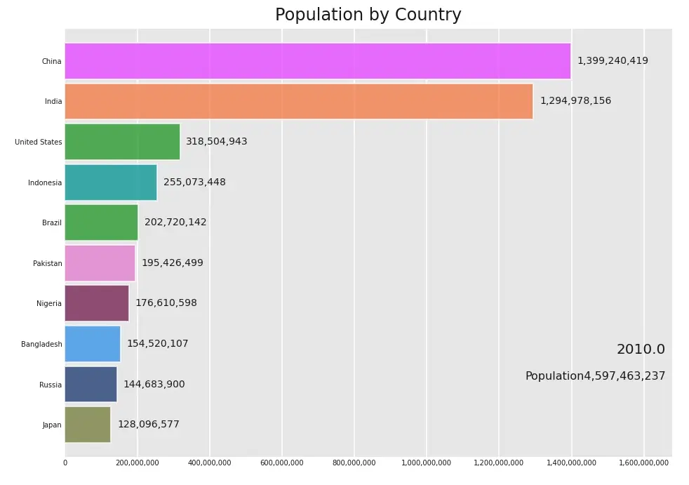
title='Population by Country',
title_size='',
bar_label_size=7,
tick_label_size=5,
shared_fontdict={'color' : '.1'},
scale='linear',
writer=None,
fig=None,
bar_kwargs={'alpha': .7},
filter_column_colors=True)
Important parameters:
-
df : pandas DataFrame: Must be a 'wide' DataFrame where each row represents a single period of time. Each column contains the values of the bars for that category. Optionally, use the index to label each time period. The index can be of any type.
-
filename : None or str, default None: If None return animation as an HTML5 string. If a string, save animation to that filename location. Use .mp4, .gif, .html, .mpeg, .mov and any other extensions supported by ffmpeg or ImageMagick.
-
n_bars : int, default None - Choose the maximum number of bars to display on the graph. By default, use all bars. New bars entering the race will appear from the edge of the axes.
-
steps_per_period : int, default 10: The number of steps to go from one time period to the next. The bars will grow linearly between each period.
-
period_length : int, default 500: Number of milliseconds to animate each period (row). Default is 500ms (half of a second)
-
bar_size : float, default .95: Height/width of bars for horizontal/vertical bar charts. Use a number between 0 and 1 Represents the fraction of space that each bar takes up. When equal to 1, no gap remains between the bars.
 World Population from 1955 to 2020